• University of Cambridge

L^AT_EX maths and graphics

Tim Love

May 11, 2012

This handout assumes that you have already read the Advanced LaTeX document.

Note that there's an alternative way of producing maths in L^AT_EX - AMS-L^AT_EX. See the for details.

If you want to more more about graphics, see by Keith Reckdahl.

Comments and bug reports to Tim Love (tl136).

Copyright © 2004-2012 by T.P. Love. This document may be copied freely for the purposes of education and non-commercial research. Cambridge University Engineering Department, Cambridge CB2 1PZ, England.

Contents

1  Maths
    1.1  Environments
    1.2  Special Characters
        1.2.1  Greek
        1.2.2  Miscellaneous
        1.2.3  Arrows
        1.2.4  Calligraphic
        1.2.5  Character Modifiers
        1.2.6  Common functions
    1.3  Subscripts and superscripts
    1.4  Overlining, underlining and bold characters
    1.5  Roots and Fractions
    1.6  Delimiters
    1.7  Numbering and labelling
    1.8  Matrices
    1.9  Macros
    1.10  Packages
    1.11  Fine tuning
    1.12  Maths and Postscript fonts
    1.13  Matlab and LaTeX
    1.14  Examples
2  Graphics
        2.0.1  psfrag: adding maths to postscript files
    2.1  Scaling, rotation, clipping, wrap-around and shadows

1  Maths

There's more to maths typesetting than meets the eye. Many conventions used in the typesetting of plain text are inappropriate to maths. L^AT_EX  goes a long way to help you along with the style. For example, in a L^AT_EX maths environment, letters come out in italics, `-' as `−' (minus) instead of the usual `-' (dash), `*' becomes *, ' becomes ′ and spacing is changed (less around `/', more around `+'). Many of the usual L^AT_EX constructions can still be used in maths environments but their effect may be slightly different; eg \textbf{  } only affects letters and numbers. `{' and `}' are still special characters; they're used to group characters. As usual in L^AT_EX you can override the defaults, but think before doing it: maths support in L^AT_EX has been carefully thought out and is quite logical though the L^AT_EX source text may not be very readable. It's a good idea to write out the formulae on paper before you start L^AT_EXing, and try not to overdo the use of the `\frac' construction; use `/' instead.

1.1  Environments

There are 2 environments to display one-line equations.

equation:-

Equations in this environment are numbered.

\begin{equation}
 x + iy
\end{equation}

x + iy

(1)

displaymath:-

These won't be numbered. \[, \] can be used as abbreviations for \begin{displaymath} and \end{displaymath}.

\begin{displaymath}
 x + iy
\end{displaymath}

x + iy

Never leave a blank line before these equations; it starts a new paragraph and looks ugly. '\displaystyle' is the font type used to print maths in these display environments. Other relevant environments are:-

math:-

For use in text. \( and \) can be used to delimit the environment, as can the T_EX constructions $ and $ . For example, $x=y^2$ gives x=y².

eqnarray:-

This is like a 3 column tabular environment. Each line by default is numbered. You can use the eqnarray* variant to suppress numbering altogether.

\begin{eqnarray}
a1 & = & b1 + c1\nonumber\\
a2 & = & b2 - c2
\end{eqnarray}

a1 = b1 + c1 a2 = b2 − c2 (2)

Maths in "display" and "inline" environments have different default sizes for some characters and other behavioural differences so that a line of maths won't impinge on text lines below or above. If you want to put some non-maths text in amongst maths then enclose it in an \mbox{...}.

1.2  Special Characters

The The Comprehensive LATEX Symbol List document offers 105 pages of symbols. Here are just a few.

1.2.1  Greek

1.2.2  Miscellaneous

1.2.3  Arrows

1.2.4  Calligraphic

These characters are available if you use the \mathcal control sequence.

 
${\mathcal A B C D E F G H I J K L M N O P Q R S T U V W X Y Z}$

gives A B C D E F G H I J K L M N O P Q R S T U V W X Y Z Also useful are "blackboard" style characters. \mathbb{ R Q Z} gives R Q Z (requires the amsfonts package).

1.2.5  Character Modifiers

Note that the wide versions of hat and tilde cannot produce very wide alternatives. The `\not' operator hasn't properly cut the following letter. The Fine Tuning section on page pageref describes how to adjust this. If you want to place one character above another, you can use \stackrel, which prints its first argument in small type immediately above the second

$ a \stackrel{def}{=} b + c $

gives See the Macros section for how to stack characters using atop.

1.2.6  Common functions

In a maths environment, L^AT_EX assumes that variables will have single-character names. Function names require special treatment. The advantage of using the following control sequences for common functions is that the text will not be put in math italic and subscripts/superscripts will be made into limits where appropriate.

\arccos	\arcsin	\arctan	\arg	\cos	\cosh	\cot
\coth	\csc	\deg	\det	\dim	\exp	\gcd
\hom	\inf	\ker	\lg	\lim	\liminf	\ln
\log	\max	\min	\Pr	sec	\sin	\sinh
\sup	\tan	\tanh

1.3  Subscripts and superscripts

These are introduced by the `^' and `_' characters. Depending on the base character and the current style, the sub- or superscripts may go to the right of or directly above/below the main character. With letters it goes to the right.

$F_2^3$

produces `F<sub>2</sub><sup>3</sup>'. Note that the sub- and superscripts aren't in line. To make them so, you can add an invisible character after the `F'. $F{}_2^3$ produces F₂³. With ∑ the default behaviour is different in display and text styles.

$\sum_{i=0}^2 $ 

produces ∑_i=0² (text style) but

\[\sum_{i=0}^2 \] 

produces (in display style)

2 ∑ i=0

This default behaviour can be overridden, if you really need to. For example in text mode,

$\sum\limits_{i=0}^2$ 

produces ∑_i=0²

1.4  Overlining, underlining and bold characters

$\underline{one} \overline{two}$ 

produces one―two. This is not a useful facility if it's used more than once on a line. The lines are produced so that they don't quite overlap the text; lines over or under different words won't in general be at the same height. To be able to reproduce bold maths, it's best to use the bm package. $E = \bm{mc^2}$ produces E = mc². Alternatively, you can use \mathbf{} to create bold characters - $\mathbf{F}_2^3$ produces F₂³. or you can use the following idea

\usepackage{amsbsy} % This loads amstext too
\begin{document}
$\omega + \boldsymbol{\omega}$

% Use the following if whole expressions need to be in bold
{\boldmath $\omega $}
\end{document}

1.5  Roots and Fractions

$\sqrt{4} + \sqrt[3]{x + y}$

gives √4 + ³√{x + y}. Three constructions for putting expressions above others are

frac:-

$\frac{1}{(x + 3)}$ produces .

choose:-

${n + 1 \choose 3}$ produces .

atop:-

${x \atop y}$ produces .

These constructions can be used with ones described earlier. E.g.,

\[ \sum_{-1\le i \le 1 \atop 0 < j < \infty} f(i,j)\]

gives

∑ [(−1 ≤ i ≤ 1) || (0 < j < ∞)]  f(i,j)

1.6  Delimiters

This table shows the standard sizes. To get bigger sizes, use these prefices

(for left delimiters)	(for right delimiters)	magnification
\bigl	\bigr	a bit bigger, but won't overlap lines
\Bigl	\Bigr	150% times big
\biggl	\biggr	200% times big
\Biggl	\Biggr	250% times big

For example,

$\Biggl\{2\Bigl(x(3+y)\Bigr)\Biggr\}$

gives . If you're not using the default text size these commands might not work correctly. In that case try the exscale package. It's preferable to let L^AT_EX choose the delimiter size for you by using \left and \right. These will produce delimiters just big enough for the formulae inbetween.

$\left( \frac{(x+iy)}{\{\int x\}} \right)$

gives The left and right delimiters needn't be the same type. It's sometimes useful to make one of them invisible

\[ z = \left\{
              \begin{array}{ll}
                   1 & (x>0)\\
                   0 & (x<0)
              \end{array}
       \right. 
\]

produces Over- and underbracing works too.

$\overbrace{\alpha \ldots \omega}^{\mbox{greek}} 
 \underbrace{a \ldots z}_{\mbox{english}}$

produces

1.7  Numbering and labelling

Numbering happening automatically when you display equations. If you don't want an equation numbered, use \nonumber beside the equation. Equation numbers appear to the right of the maths by default. To make them appear on the left use the leqno class option (i.e., use \documentclass[leqno,....]{....}). Use \label{} to label an equation (or figure, section etc) in order to reference from elsewhere.

\begin{equation}
W_{\bf S}(t,\omega) = \int\limits_{-\infty}^{\infty} {
  {\cal R}_{\bf S}(t,\tau) e^{-j\omega\tau} \,d \tau }
\label{LABELLING}
\end{equation}

Now the following text

 refers back to equation \ref{LABELLING}

refers back to equation 3 by number, and

 
 refers back to the equation on page \pageref{LABELLING}

refers back to the equation on page pageref. A file will have to be L^AT_EX'ed twice before the references, both forwards and backwards, will be correctly produced.

1.8  Matrices

The array environment is like L^AT_EX's tabular environment except that each element is in math mode. The number and alignment of columns is controlled by the arguments - use l, c or r to represent each column with either left, center or right alignment. The default font style used is \textstyle but you can override this by changing the \displaystyle.

\begin{math}
\begin{array}{clrr} %
      a+b+c & uv & x-y & 27 \\
       x+y  & w  & +z  & 363 
\end{array}
\end{math}

produces

a+b+c	uv	x−y	27
x+y	w	+z	363

The rows are arranged so that their centres are aligned. You can align their tops or bottoms instead by using a further argument when you create the array.

\begin{array}{clrr}[t]

would produce top-aligned lines, and `[b]' would produce bottom-aligned ones. The Delimiters section of this document shows how to bracket matrices. T_EX has a few maths facilities not mentioned in the L^AT_EX book. The following T_EX construction might be useful.

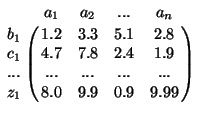
\begin{math}
\bordermatrix{&a_1&a_2&...&a_n\cr
          b_1 & 1.2  & 3.3  & 5.1  & 2.8  \cr
          c_1 & 4.7  & 7.8  & 2.4  & 1.9  \cr
          ... & ...  & ...  & ...  & ...  \cr
          z_1 & 8.0  & 9.9  & 0.9  & 9.99  \cr}
\end{math}

1.9  Macros

These aid readability, save on repetitive typing and offer ways of producing stylistic variations on standard L^AT_EX formats.

\def\bydefn{\stackrel{def}{=}}
\def\convf{\hbox{\space \raise-2mm\hbox{$\textstyle  
    \bigotimes \atop \scriptstyle \omega$} \space}}

produce =^def and [( ⊗) || ( ω)]_endtextstyle when $\bydefn$ and $\convf$ are typed.

1.10  Packages

The following packages may be of help - (easy block matrices), (easy equations), (easy matrices), (easy tables), (easy vectors), (nested arrays), (gives more choice in theorem layout), subeqnarray (Renumbering of sub-arrays in math-mode), subeqn (Different numbering sub-arrays).

1.11  Fine tuning

It's generally a good idea to keep punctuation outside math mode; L^AT_EX's normal handling of spacing around punctuation is suspended during maths. Sometimes you might want to adjust the spacing in a formula (e.g., you might want to add space before dx). Use these symbols :-

a\, b	(a b) thin space
a\> b	(a b) medium space
a\; b	(a  b) thick space
a\! b	(a b) negative thin space

Long math expressions aren't broken automatically unless you use the package, which is still a little experimental. In an eqnarray environment you may want to break a long line manually. You can do this by putting

y & = & a + b \nonumber \\
  &   & + k

to give

y = a + b + k (4)

but the spacing around the `+' on the 2nd line is wrong because L^AT_EX thinks it's a unary operator. You can fool L^AT_EX into treating it as a binary operator by inserting a hidden character.

y & = & a + b \nonumber \\
  &   & \mbox{} + k

gives

y = a + b + k (5)

You can use the \lefteqn construction to format long expressions so that continuation lines are differently indented.

\begin{eqnarray}
\lefteqn{x+ iy=}\\
 & & a + b + c + d + e + f + g + h + i + j + k +\nonumber\\
 & & l + m \nonumber
\end{eqnarray}

x+ iy= (6) a + b + c + d + e + f + g + h + i + j + k + l + m

If you want more vertical spacing around a line you can create an invisible vertical ßtruct" in LaTeX. creates a box of width 0, height 1cm which starts .3cm below the usual line base, use \rule[-.3cm]{0cm}{1cm}. By adjusting these values you should be able to create as much extra space below/above the maths as you like. "[A/B] and" is created by

$A \over B$  \rule[-.3cm]{0cm}{1cm}{and}

1.12  Maths and Postscript fonts

It's easy to use a postscript font (like helvetica) for the text of a L^AT_EX document. What's harder is using the same font for maths - the font will lack many of the special characters required for maths. An easy, reasonable option is to use the mathptmx package to put the maths into the postscript Times and symbol fonts where possible. Alternatively, use

• the mathpazo package (loads Palatino as the text font family and a mixture of the Pazo and CM fonts for math).
• the mathpple package (loads Palatino as the text font family and a mixture of artificially obliqued Euler fonts and CM fonts for math).

Commercial and free alternatives are under development. See Stephen G. Hartke's for details.

1.13  Matlab and LaTeX

has some support for LaTeX production. For example

  latex('(sin(x)+2*x+3*x^2)/(5*x+6*x^2)','math.tex')

puts the LaTeX representation of the expression into a file called math.tex. Type "help latex" inside matlab for details.

1.14  Examples

• \begin{eqnarray}
  {\cal M}^2(\hat{\theta},\theta) &=& E[(\hat{\theta} - \theta)^2]
  \nonumber \\
  {\cal M}^2(\hat{\theta},\theta) &=& {\rm var}^2(\hat{\theta}) + 
  {\cal B}^2(\hat{\theta}).
  \end{eqnarray}
  
  

  gives
  

  M2( ^ θ   ,θ) = E[( ^ θ   − θ)2] M2( ^ θ   ,θ) = var2( ^ θ   ) + B2( ^ θ   ). (7)

• \begin{equation}
  \hat{W}_{s}(t,\omega;\phi) \bydefn 
  \int\limits_{-\infty}^{\infty} 
  {\hat{\cal R}_s(t,\tau;\psi) e^{-j\omega \tau}
  \, d \tau }
  \end{equation}
  
  

  gives
  

  ^ W   s  (t,ω;ϕ) def =   ∞ ⌠ ⌡ −∞  ^ ℜ   s  (t,τ;ψ)e−jωτ d τ

  (8)

• \begin{eqnarray}
  {\cal B}(t,\omega) & \approx &
  {1 \over 4\pi}
  {\cal D}_t^2 W_{\bf S}(t, \omega)
  {{{\scriptstyle \infty} \atop
  {\displaystyle \int \! \int \!
  }}\atop {\scriptstyle -\infty}}
  t_1^2
  \phi(t_1,\omega_1) \, dt_1 d\omega_1
  \nonumber \\
  && +
  {1 \over 4\pi}
  {\cal D}_\omega^2 W_{\bf S}(t, \omega)
  {{{\scriptstyle \infty} \atop
  {\displaystyle \int \! \int \!
  }}\atop {\scriptstyle -\infty}}
  \omega_1^2
  \phi(t_1,\omega_1) \, dt_1 \, d\omega_1.
  \label{F4}
  \end{eqnarray}
  
  

  gives
  

  B(t,ω) ≈ 1 4π Dt2 WS(t, ω) ∞ ⌠ ⌡ ⌠ ⌡ −∞ t12ϕ(t1,ω1)  dt1 dω1 + 1 4π Dω2 WS(t, ω) ∞ ⌠ ⌡ ⌠ ⌡ −∞ ω12ϕ(t1,ω1)  dt1  dω1. (9)

• \newsavebox{\DERIVBOXZLM}
  \savebox{\DERIVBOXZLM}[2.5em]{$\Longrightarrow\hspace{-1.5em}
  \raisebox{.2ex}{*}
  \hspace{-.7em}\raisebox{-.8ex}{\scriptsize lm}\hspace{.7em}$}
  \newcommand{\Deriveszlm}{\usebox{\DERIVBOXZLM}}
  
  \Deriveszlm
  
  

  gives
  ⇒*lm  

2  Graphics

Graphics can be produced

• from within LaTeX - pictures can be drawn in a picture environment, but you'll find graph paper handy (xfig can create code for the picture environment). The pstricks packages is far more powerful.
• by any program that can produce Postscript files (for LaTeX) or JPEG, PNG andPDF (for pdflatex).

Whatever graphics you want to add, you should use the figure environment so that L^AT_EX can cope sensibly with situations where, for example, you attempt to insert near the bottom of a page a graphic that's half a page high. The figure environment will float the graphic to the top or bottom of the page, or on the next page, or here (where you asked for it).

h	here
t	top of page
b	bottom of page
p	on a page with no text

The order you put these letters in doesn't matter, but whether you include them does. Putting ! as the first argument in the square brackets will encourage L^AT_EX to do what you say, even if the result's sub-optimal. Below is a simple (and usually sufficient) usage. See the online hints for further details.

\begin{figure}[htbp]
   \vspace{0.5in}
   \caption{0.5 inch of space}
\end{figure}

It's possible to have more than one graphic in a figure. See the example later on.

pdflatex supports JPEG, PNG andPDF images - but not postscript. latex supports Postscript files as long as they have a proper bounding box comment; i.e. L^AT_EX requires full

2.0.1  psfrag: adding maths to postscript files

Many packages that produce postscript output don't provide good maths facilities. It's often easier to add the maths in later using the psfrag package. This lets you replace text in a postscript file (produced with xfig, matlab, etc) by a fragment of L^AT_EX. For example, doing

\usepackage{psfrag}
...
\begin{figure}
\psfrag{MATHS}{$x^2$}
\includegraphics{foo.eps}
\end{figure}

would display the file with MATHS replaced by x². See the psfrag documentation for details.

2.1  Scaling, rotation, clipping, wrap-around and shadows

The graphicx package includes routines that are useful even without graphics. \reflectbox{Reflect} produces and \resizebox{3cm}{0.2cm}{Stretched} produces . To scale imported graphics, use some optional arguments

   \includegraphics[width=5cm,height=10cm]{yourfile.jpg}

would rescale the postscript so that it was 5cm wide and 10cm high. To make the picture 5cm wide and scale the height in proportion use

   \includegraphics[width=5cm]{yourfile.png}

To rotate anticlockwise by the specified number of degrees, use

   \includegraphics[angle=150]{yourfile.pdf}

These options can be combined - note that order matters. The following examples demonstrate how to combine these features and how to use the subfig package to have more than one graphic in a figure.

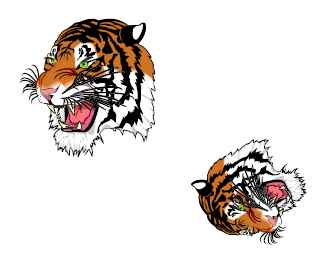
\centering
\begin{figure}[hbtp]
  \includegraphics[height=40mm]{tiger.jpg} 
  \includegraphics[angle=120, height=20mm]{tiger.jpg} 
\caption{Tigers}
\end{figure}

% remember to do \usepackage{subfig} at the top of the document! 
\begin{figure}[hbtp]
\centering
\subfloat[Small]% \quad on the next line adds spacing
{\includegraphics[height=30mm]{tiger.jpg}}\quad
\subfloat[Medium]
{\includegraphics[width=40mm]{tiger.pd}}\quad
\subfloat[Large]
{\includegraphics[height=50mm]{tiger.jpg}} 
\caption{3 crests}
\end{figure}

To clip images use the viewpoint argument. The following fragment would display only part of the image. The viewport coordinates are in the same units as the bounding box.

\begin{figure}[htbp]
\includegraphics[viewport=200 400 400 600,width=5cm,clip]%
{tiger.jpg}
\end{figure}

% Use the floatflt package
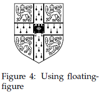
\begin{floatingfigure}[l]{4cm}
\includegraphics[width=2cm]{tiger.jpg}  
\caption{Using floatingfigure}
\end{floatingfigure}

Figure 4: Using floatingfigure

The package lets you insert a graphic and have the text wrap around it. You can provide 2 arguments to the floatingfigure command: the first (l or r) selects whether you want the graphic to be on the left or right of the page. The 2nd argument gives the width of the graphic. Not all text will flow perfectly around (for example, verbatim text fails, as illustrated below) so check the final output carefully.

Using the fancybox package gives you access to \shadowbox, \ovalbox, \Ovalbox and \doublebox commands, which can be used with text or with graphics. For example, \shadowbox{shadow package} produces and

\ovalbox{\includegraphics[height=10mm]{crest.jpg}}

produces . Unfortunately, the fancybox package as supplied suppresses the table of contents. The locally produced contentsfancybox solves this, but may introduce graphics problems.

---

File translated from T_EX by T_TH, version 4.03.
On 11 May 2012, 11:47.